
Author(s)

This testimony was delivered before the U.S. House of Representatives Committee on Ways and Means Subcommittee on Select Revenue Measures on July 30, 2014.
Introduction
Chairman Tiberi, Ranking Member Neal, and Members of the Committee, thank you for inviting me to present my views on the importance of dynamic analysis. In my remarks, I plan to discuss why dynamic analysis is important, comment on several recent dynamic analyses of the Tax Reform Act of 2014 (TRA 2014), discuss how TRA 2014 could be changed to enhance the projected increases in economic growth, and comment on how to implement dynamic analysis to improve the budget process.
Why Dynamic Analysis Is Important
A popular management adage is, “If you can’t measure it, you can’t manage it.” Dynamic analysis provides valuable information about the effects of policy proposals on economic growth, and it is important that we use this information to better manage US fiscal policy. In fact, routinely disregarding information on the macroeconomic effects of alternative proposals leads to a budget process that undervalues proposals that help grow the economy and overvalues proposals that shrink the economy. We can no longer afford a budget process that fails to maximize economic growth.
Dynamic analysis allows the budget process to account for the effect of policy proposals on the level of gross domestic product (GDP), which is a function of the size of the capital stock and total hours of work in the economy. In addition, dynamic analysis may be used to examine the effects of policies on wages, consumption, welfare (for certain types of models), distributional outcomes (both within and across generations), as well as other important variables. While dynamic analysis will provide valuable information about the relative economic effects of alternative policies, it will not solve the fiscal crisis facing the United States. Policymakers will still face many tough decisions. In addition, it is important to note that preparing a dynamic analysis is no easy task and presenting and communicating the results to members, their staff, and the general public is also difficult.
Implementing a budget process that encourages the adoption of pro-growth, fair, and simple tax and spending policy reform is critical given that current fiscal policies are projected to lead to larger budget deficits and dramatic long-run increases in the debt-to-GDP ratio, especially if the sluggish rebound in economic growth over the last several years continues.
Note that dynamic analysis is already used on a fairly wide scale. For example, the Joint Committee on Taxation (JCT) has produced dynamic analyses of several significant tax proposals (JCT, 2003; JCT, 2005; JCT, 2006; JCT, 2014a; JCT, 2014b). In addition, the Department of the Treasury’s Office of Tax Analysis (OTA) has published dynamic analyses of the reform proposals made by the President’s Advisory Panel on Federal Tax Reform (Carroll, Diamond, Johnson, and Mackie, 2006) and the proposal to permanently extend the President’s tax relief (OTA, 2006). The Congressional Budget Office also publishes macroeconomic analyses of various proposals, including the President’s Budget (CBO, 2003a and 2003b).
Dynamic Analysis of TRA 2014
TRA 2014 was a comprehensive proposal for reform of both the corporate and personal income tax systems. The corporate income tax (CIT) reform was structured as a traditional base-broadening, rate-reducing (BBRR) reform. The plan would have lowered the CIT rate to 25 percent, phased in over five years, and eliminated a variety of business tax preferences, including accelerated depreciation (so that tax depreciation would approximate economic depreciation), expensing of research and development costs and half of advertising costs, and the deduction for domestic production. The plan would have not allowed the last-in first-out (LIFO) inventory accounting rule and would have permanently created a 15 percent tax credit for research and development expenses.
The reform also changed the treatment of foreign source income, including moving to a 95 percent participation exemption (territorial) system. The effective tax rate is roughly 1.25 percent with a 25 percent CIT rate. It also allowed for current taxation of foreign source income from intangibles, defined as income in excess of 10 percent on basis in depreciable assets (excluding other subpart F income and commodities income) due to foreign sales at a minimum tax rate of 15 percent (25 percent for US sales), subject to foreign tax credits. The 15 percent rate also applied to intangibles income (income in excess of 10 percent on basis in depreciable assets other than from commodities) on sales to foreign markets from the United States. The reform would have limited subpart F income to low-taxed income and created a minimum tax of 12.5 percent for foreign sales and active financial services income, in addition to the minimum tax rates noted above. There was also a one-time tax on the stock of unrepatriated profits, at an 8.75 percent rate on cash and equivalents and at a 3.5 percent rate on illiquid assets.
The plan would have also reformed the tax treatment of individual income by broadening the tax base and lowering the rates on individual income. It would have included a 10 and 25 percent rate bracket, with a 10 percent surtax on high income households (above $450,000 for married couples). The standard deduction, child credit, and the 10 percent bracket were phased out for high-income households. The plan would have repealed itemized deductions for state and local (non-business) taxes, medical expenses, personal exemptions, and the alternative minimum tax. In addition, it would have limited the mortgage interest deduction. Capital gains and dividends would have been taxed as normal individual income after a 40 percent exclusion.
The Diamond-Zodrow (DZ) computable general equilibrium model was used to simulate the effects of TRA 2014. The model is structured so that consumers choose consumption, labor supply, and saving to maximize welfare over their lifetimes. The model includes 55 adult generations (intended to capture an adult’s working life from age 23 to 78) alive at any point in time, and is thus typically described as an overlapping generations model. Firms choose labor demand and the time path of investment to maximize profits, subject to adjustment costs. The model includes five different production sectors, including a multinational corporation (MNC), a domestic corporation, a non-corporate (pass-through) firm, and owner and rental housing sectors. In addition, the corporate firms have a variable debt-to-equity ratio. The government uses corporate and personal income taxes to finance a fixed level of government services. The model must begin and end in a steady-state equilibrium with all key macroeconomic variables growing at an exogenous growth rate (which equals population plus productivity growth). The model is calibrated to roughly match the US economy in a given base year.
The model includes domestic and foreign MNCs (parents and subsidiaries) with highly mobile firm-specific capital (FSK) that earns above normal returns, and relatively immobile ordinary capital that earns normal returns. This approach follows Becker and Fuest (2011) who argue that differential capital mobility is an important part of modeling international capital flows. All of the multinational corporations — the US parent firm and its foreign-based subsidiary, and the foreign-based rest of the world parent firm and its US subsidiary — are assumed to have analogous production functions. The modeling approach we utilize generally follows the approach for firm-specific capital developed by de Mooij and Devereux (2009) and Bettendorf, Devereux, van der Horst, Loretz, and de Mooij (2009). The MNC is assumed to own a unique firm-specific production input (FSK), such as patents or other proprietary technology, brand names, and good will, coupled with unique managerial skills and knowledge of production processes, which allows it to permanently earn above-normal returns. This firm-specific factor is treated as “quasi-fixed,” as it is assumed to be fixed in total supply in any given period, but this fixed amount can be reallocated across the US and the rest of the world. The main role of this assumption is to determine the fraction of production using FSK that occurs in the US relative to the rest of the world. The elasticity of FSK (in terms of its location) with respect to the tax rate differential is assumed to be 8.6, which is calculated from the assumption that the capital-share-weighted aggregate portfolio elasticity of all capital (both FSK and ordinary capital) is 3.0. Assuming a relatively small portfolio elasticity of 0.5 for ordinary capital implies an elasticity of 8.6 for FSK. The basic idea is that the location decision of where to use FSK is highly elastic with respect to the tax rate differential, although we do phase in over time the reallocation of production involving FSK in response to changes in relative taxes. In addition, MNCs engage in income shifting that depends on the tax differential between the United States and the rest of the world, including tax havens. MNCs must make a repatriation decision and are subject to a residual US tax on repatriations. The model includes foreign trade, international capital mobility, and foreign ownership of domestic capital. Ordinary capital (capital that earns a normal rate of return) is disaggregated into structures, equipment, and inventories.
Simulation Results: Economic Effects of TRA 2014
Diamond-Zodrow Results
Table 1 shows the Diamond-Zodrow analysis of TRA 2014, which was prepared for the Business Round Table (BRT). The most important factor is the reduction in income shifting as the CIT rate declines. In addition, other important factors include the move to territorial, the more efficient allocation of capital, and the reallocation of FSK. DZ find that TRA 2014 would increase GDP by 1.2 percent after five years, by 2.2 percent after 10 years, and by 3.1 percent in the long run. The long-run increase in GDP is primarily driven by a 5.0 percent increase in the ordinary capital stock and a 0.3 percent increase labor supply. In the long run, a 57 percent reduction in income shifting allows the CIT rate to decline an extra 5 percentage points to 19.9 percent.
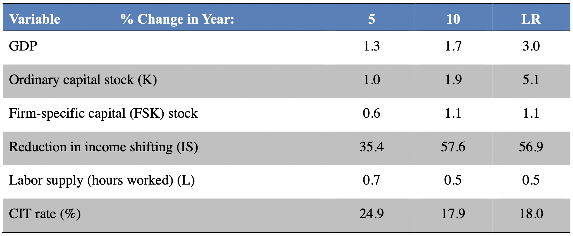
The DZ model includes differential capital mobility by having one capital good that is relatively immobile and another capital good that is assumed to be highly mobile. An important question is how did this assumption affect the reported results. Table 2 shows the effects of adopting TRA 2014 under the assumption that all capital is relatively immobile (both capital goods have an elasticity of 0.5 with respect to the tax rate differential). In this case, GDP increases by 1.3 instead of 1.2 percent five years after reform, by 1.7 percent instead of 2.2 percent 10 years after reform, and by 3.0 instead of 3.1 percent in the long run. Without differential mobility FSK increases by 0.6 percent and 1.1 percent in the long run instead of 16.3 and 23.5 percent. The labor supply increase is slightly higher in this case. This demonstrates that the addition of FSK is not driving the results in the DZ analysis. Although the reallocation of FSK to the US increases production of the good produced by the US multinational, the GDP effects of this reallocation are offset by other factor reallocations, especially a return of ordinary capital to the rest of the world.
Table 1 — Diamond-Zodrow Analysis of Camp for BRT
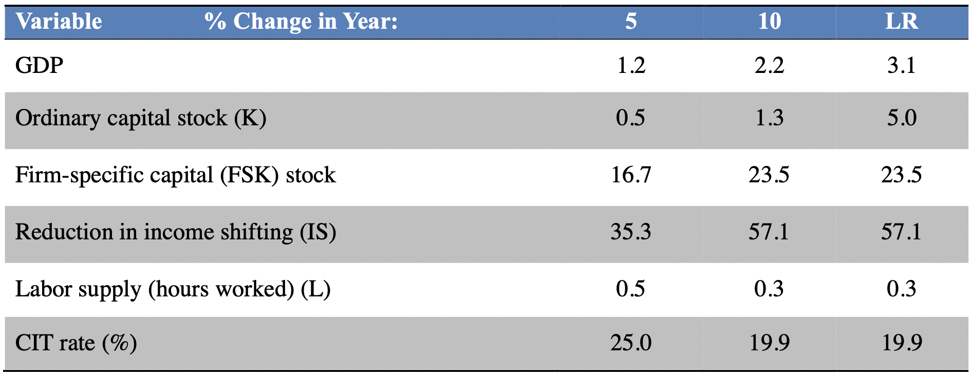
Table 2 — Diamond-Zodrow Analysis of Camp with Immobile FSK
JCT Results
The JCT analysis used two models, the MEG model and the OLG model, which is based on the DZ model. Comparing JCTs OLG results with the DZ results show that the results differ significantly. While the GDP results are roughly similar initially, the results published by JCT decline during the budget window, while the DZ results increase during the budget window and into the long run. In addition, comparing the results shows that JCT found large labor supply effects and smaller and declining capital stock effects, while DZ found small labor supply effects and positive and increasing capital stock effects.
However, even though DZ and JCT used the same model, there were several significant differences that help explain the differences in the results. The two main differences are:
-
JCT assumes that the initial level of CIT revenues lost due to income shifting is 20 percent of the current CIT base, not 24 percent as in DZ.
- JCT assumes that any excess revenues go to increasing government transfers, rather than further CIT rate reductions, as in DZ.
Both assumptions are critical, as the reduction in income shifting is an important driver of the results in the DZ analysis. Larger amounts of initial shifting allows for a larger reversal of income shifting as the US reduces its CIT rate. Further rate reductions enhance this effect as the associated decline in income shifting allows further rate reduction that is obtained without the negative effects of base broadening. An additional difference is that DZ accounts for the negative impact of base broadening on real wage rates and thus on labor supply in the model (that is, the effect of base broadening on consumer prices, e.g., elimination of deductions for state and local taxes and limitation of charitable contributions effectively increases consumer prices and thus reduces the real after-tax wage), which offsets some of the positive impact of rate reductions; JCT does not include this effect in the model but may account for it in its calculation of effective tax rates. Finally, there are also some differences in parameter values.
Tax Foundation Results
The Tax Foundation found much smaller results, with only a 0.2 percent increase in GDP in long run. The small size of its result is attributable primarily to a reduction in the capital stock of 0.2 percent as the cost of capital increases under TRA 2014. The Tax Foundation predicted that labor supply would increase by 0.5 percent. But, the Tax Foundation analysis discusses but then ignores the benefits of reduced income shifting, the benefits of reallocation of firm-specific capital to the United States, and the benefits of moving to a territorial system. DZ included these important factors in modeling the effects of TRA 2014, which helps explain the differences in the results.
For example, using the DZ model and simulating the effects of a similar (base broadeners are slightly different) CIT reform (but no individual income tax reform) while ignoring the three factors above produces significantly negative effects with GDP down 1.7 percent in long run, and a CIT rate reduction to only 31.4 percent. This illustrates the powerful effects on GDP of reversing income shifting and using the revenue gains from reform to further lower the corporate income tax rate.
Enhancing the Economic Growth Effects of TRA 2014
There are several lessons that can be drawn from these simulations. First, a BBRR reform that repeals targeted investment incentives — such as eliminating accelerated depreciation or other incentives that affect investment at the margin — to finance rate reductions grants a windfall gain to existing capital by reducing the tax rate applied to such capital, with the windfall exacerbated by the existence of above normal rates of return. The resulting increase in the cost of capital reduces investment and output, and makes it much less likely that a BBRR reform will result in positive macroeconomic effects in both the short and long run.
Second, the international considerations stressed above make it more likely that a BBRR reform will generate positive macroeconomic effects. A reduction in the statutory corporate income tax rate will result in a reallocation of highly mobile firm-specific capital that earns above-normal returns to the United States — although this effect is offset to a significant extent by other general equilibrium effects, including the return of ordinary capital to the rest of the world and a reduction in labor supply. More importantly, a reduction in the statutory corporate income tax rate reverses some income shifting from the United States, which provides a “free” source of revenue — effectively a CIT rate cut without the costs of base broadening — that significantly increases the benefits of a BBRR reform. In addition, the changes in trade that accompany a reversal of income shifting also have important effects, increasing net exports and thus output. Note, however, that the amount of income shifting in the initial equilibrium, as well as the extent of the reversal of this income shifting with a reduction in the CIT rate in the United States, are open to debate, and that the macroeconomic benefits of a BBRR reform would be significantly reduced if the extent to which income shifting is reversed with US CIT rate cuts were smaller than assumed in the simulations.
Third, although the simulations indicate that the net macroeconomic effects of the particular territorial tax reform analyzed are positive, the gains from such a reform are fairly modest. This is not surprising: since the current worldwide tax system — which taxes foreign source income only when repatriated and allows foreign tax credits (including cross-crediting of taxes from high-tax countries against income from low-tax countries) — imposes a very low residual US tax rate on repatriations, switching to a territorial system is likely to have relatively limited macroeconomic effects.
The net effect of all these factors implies that the macroeconomic effects of a BBRR CIT reform depend very much on both the details of the specific reform proposal and the context in which it is imposed. These results indicate that a BBRR CIT reform is more likely to result in positive macroeconomic effects if (1) the initial amount of income shifting is large and is reduced significantly when the statutory CIT rate in the US declines, (2) accelerated depreciation is retained instead of being used as a base broadening provision, and (3) the BBRR reform includes a move to a territorial system of the type analyzed in the report, that is, one that includes anti-base erosion provisions that are sufficiently effective that the tax sensitivities of international capital and income shifting are the same as prior to the enactment of the reform.
BBRR individual income tax reform can also increase GDP. The magnitude of the gains depends on the reduction of individual income tax rates, the reduction of capital gains and dividends tax rates (if treated separately such as under a dual income tax), and the base broadeners that are used to finance the rate reductions. In addition, an important factor is how much individual income tax rate reduction is financed by base broadening in the corporate sector.
Implementing Dynamic Analysis to Improve the Budget Process
As noted above, dynamic analysis has already been used on a wide scale. However, there are a number of important issues regarding how to use dynamic analysis to improve the budget process.
One of the primary goals of dynamic analysis should be to compare the macroeconomic effects of various provisions. If the sole focus is measuring the economic effects of a base reform proposal for the sole purpose of determining the revenue feedback, then much of the additional information that could be gleaned from dynamic analysis would not be realized. Obviously, analyzing every provision separately would be counterproductive, as this would be an overwhelming burden on staff resources. However, dynamic analysis should be used to compare alternative proposals, which will require more flexibility and foresight in the timing of the legislative process.
Dynamic analysis should examine and present results on the effects of groups of related provisions separately from the entire proposal for large policy reforms. For example, it would be informative to break TRA 2014 into three dynamic analyses examining the effects of corporate tax reform, a move to territorial, and the effects of the individual income tax reforms (and it may be of interest to break these apart as well). Providing estimates of parts of larger reforms would allow for more outside feedback and analysis and would reduce the extent to which the results seem to emanate from a “black box.” In addition, it may be informative to examine the effects of groups of provisions on major economic aggregates, including employment and wage income, capital, consumption, and potentially welfare. Providing disaggregated analyses would increase the reliability of the work and potentially help highlight the winners and losers of policy changes.
While examining every provision on its own would be impossible, there may be times when it makes sense to examine a single provision. For example, analyzing all current tax expenditures in a single piece of legislation would not be likely to get a dynamic analysis. However, examining each independently allows for a dynamic analysis on proposals that may have a substantial impact. Recently, JCT provided a dynamic analysis of the effects of permanently extending the provision allowing 50 percent bonus depreciation and found that it would increase GDP by 0.2 percent over the budget window and would increase the business capital stock by 0.6 to 1 percent over the budget window. Note that a temporary extension of this provision would have different economic effects and such an analysis would be of interest. However, we must avoid only analyzing proposals with positive economic effects and not analyzing proposals with negative economic effects.
Debt service costs in both the short and long runs are generally included in dynamic analysis but are not included in conventional cost or revenue estimates. This is important because budget gimmicks within the budget window can obscure the long-run effects of policies, especially policies that are debt-financed and temporary. The effects of increasing the debt should also be examined for spending policy reforms.
Dynamic analysis should also be applied to spending proposals. However, the demand-side effects of spending and tax proposals should not be considered, especially for permanent proposals. In cases in which the purpose of the policy is purely to impact short-run demand, the long-run effects of debt financing such expenditures should be carefully examined.
Macroeconomic aggregates are not the only information that should be provided to policymakers. Some measure of economic well-being should be provided in addition to the macroeconomic aggregates. This is important because positive macroeconomic effects can be associated with negative welfare effects for US residents (Diamond and Viard, 2008). Dynamic analysis of distributional effects are also often of interest both within income groups and across generations for certain proposals.
The extent of the uncertainty contained in a dynamic analysis must be acknowledged. For example, this would include discussing the sensitivity of the results to various assumptions about parameter values, the assumptions underlying the economic model, whether the policy was financed by changes in government spending (and the effects of such spending on welfare), taxes, or government debt, and assumptions about the reactions of other entities such as the Federal Reserve, state governments, and foreign countries.
Dynamic analysis should be timely so that it can be used effectively in the formulation of policy. The current House rule (XIII.3) requires an analysis of the macroeconomic effects before the bill can be considered on the floor. This is somewhat late in the political process, as many of the major details of a bill are typically established at this point. It is important to note that there are possible logistical constraints on this issue, given the current state of macroeconomic modeling.
Public disclosure is imperative and as much information as possible should be released to the public. At a minimum, enough information should be released so that outside entities could replicate the work. This will ensure that the process is seen as fair and open and will serve as a check on those who provide the estimates.
References
Becker, Johannes and Clemens Fuest. 2011. “Optimal Tax Policy when Firms are Internationally Mobile.” International Tax and Public Finance 18 (5), 580–604.
Bettendorf, Leon, Michael P. Devereux, Albert van der Horst, Simon Loretz, and Ruud de Mooij. 2009. “Corporate Tax Harmonization in the EU.” CPB Discussion Paper 133, CPB Netherlands Bureau for Economic Policy Analysis.
Carroll, Robert, John Diamond, Craig Johnson, and James Mackie III. 2006. “A Summary of the Dynamic Analysis of the Tax Reform Options Prepared for the President’s Advisory Panel on Federal Tax Reform.” U.S. Department of the Treasury, Office of Tax Analysis. Prepared for the American Enterprise Institute Conference on Tax Reform and Dynamic Analysis, May 25.
Congressional Budget Office. 2003a. “An Analysis of the President's Budgetary Proposals for Fiscal Year 2004.” March 2003.
Congressional Budget Office. 2003b. “How CBO Analyzed the Macroeconomic Effects of the President's Budget.” July 2003.
de Mooij, Ruud, and Michael P. Devereux. 2009. “Alternative Systems of Business Tax in Europe: An Applied Analysis of ACE and CBIT Reforms.” Taxation Studies 0028, Directorate General Taxation and Customs Union, European Commission.
Diamond, John W., and Alan D. Viard. 2008. “Welfare and Macroeconomic Effects of Deficit–Financed Tax Cuts: Lessons from CGE Models.” In Viard, Alan D. (ed.), Tax Policy Lessons from the 2000s (The AEI Press: Washington, DC), 145–193.
Joint Committee on Taxation. 2003. “Macroeconomic Analysis of H.R. 2, the Jobs and Growth Reconciliation Tax Act of 2003.” Congressional Record, May 08.
Joint Committee on Taxation. 2005. “Macroeconomic Analysis of Various Proposals to Provide $500 Billion in Tax Relief,” JCX-4-05. March 1.
Joint Committee on Taxation. 2006. “Macroeconomic Analysis of a Proposal to Broaden the Individual Income Tax Base and Lower Individual Income Tax Rates,” JCX-53-06. December 14.
Joint Committee on Taxation. 2014a. “Macroeconomic Analysis of the Tax Reform Act of 2014,” JCX-22-14. February 26.
Joint Committee on Taxation. 2014b. “Macroeconomic Analysis for Bonus Depreciation Modified and Made Permanent,” July 3.
U.S. Department of the Treasury, Office of Tax Analysis. 2006. “A Dynamic Analysis of Permanent Extension of the President’s Tax Relief,” July 25.


