
Introduction
Since its inception in 1935, the financial stability of the Social Security program has shown considerable sensitivity to fluctuating demographics. Much of the program’s demographic risk exposure results from its design, which finances current beneficiaries through current contributions in a so-called pay-as-you-go (PAYG) system. Because of this design, demographic changes will always cause transitory imbalances in the program, prompting policymakers to build reserves or modify the policy parameters. Understanding how to shift resources in response to demographic transitions is key to operating the program efficiently.
The Social Security Trust Fund (SSTF) serves as the program’s budgeting arm that collects revenues, manages disbursements, and holds reserves to promote the pension’s long-term financial stability. In preparation for the impending demographics-driven surge in benefit outlays as baby boomers reach retirement, policymakers have been raising revenues in excess of contemporaneous expenditures to grow the SSTF. Unfortunately, these resources will eventually exhaust, as the SSTF is projected to become insolvent in the year 2037.1 This leaves policymakers in a situation where they will need to reduce costs, increase revenue, or some combination of each.
Policymakers have at least a few options to stabilize the SSTF. Reducing benefits and increasing taxes are two conventional solutions. Other solutions include narrower cost-of-living adjustments (COLAs) and increases in the normal retirement age—the age at which retirees would begin receiving their full benefits. Scheduled increases in the normal retirement age are currently phasing in, but they not large enough to bring the SSTF into solvency.
Given that policymakers will eventually need to decide how to resolve the program’s projected shortfall, this paper presents a simulation-based approach to evaluating the conventional alternatives of adjustments to benefits or taxes. The key advantage to this method is the ability to quantify the insurance value of the benefit versus the costs of taxation, taking into account factors like declining birth rates, increases in life expectancy, and even the behavioral distortions induced by alternative policies. A declining birth rate results in a declining tax base, which raises the cost of financing any fixed benefits. Rising life expectancy increases the program’s outlays, further increasing the costs of maintaining stable benefits. Each of these cases shifts the balance between the costs and benefits of the program, which the simulation model is designed to evaluate.
Historical Overview
Social Security was not the first program of its kind in the US. The Civil War Pensions program had been running for nearly 60 years by 1935, as well as the pension plans of many states. Still, large portions of the elderly population were left without financial security. A rising poverty problem among that group hit a boiling point during the Great Depression when a large share of the elderly population was left without sufficient resources to provide for themselves. Several state- and federal-level proposals began appearing in response, including the Townsend Plan and a program proposed by the General Welfare Federation of America. While these plans offered monthly monetary support to older workers, they heavily restricted the use of the money and limited who was covered by the provisions. Although these plans were initially successful at highlighting the growing problem of elderly poverty, they could not garner enough support to be widely implemented. The demands for an effective solution were finally met with the passing of the Social Security Act of 1935.
What was unique about the 1935 Social Security Act was its breadth: while other programs had their efficacy limited either by restrictive qualifications or small geographical coverage, Social Security was designed to cover all U.S. citizens over the age of 65 with monthly benefits based on their lifetime earnings. The act also provisioned for assistance to dependent children, blind citizens, and both maternal and child healthcare, in addition to funding for rehabilitation programs designed to bring disabled workers back into employment.2
While broad for its era, the program lacked many features that we today associate with Social Security. One of the most notable expansions of the bill took place in 1939 with the addition of both survivor’s and dependent insurance, extending a worker’s benefits to their spouses and children and providing a safety net in the case of their premature death.3 Though blind workers were covered by the 1935 act, broader disability insurance would not be addressed until the 1950s with the addition of disability freezes to preserve average earnings after an injury and benefit eligibility for disabled seniors. The latter would later be expanded to all disabled adults by 1960.
Amidst all of this expansion, there was one feature that notably was not growing: benefits. Once benefit value was determined, retirees and other covered individuals would receive that same benefit until the end of their life. Consequently, persistent inflation eroded the real value of Social Security benefits to nearly half of their initial levels. In response, amendments were passed in 1950 that created the framework for COLAs designed to keep up with rising prices. All benefits saw an immediate 77% increase at this time, and from that point on, biennial adjustments of 10-14% were passed to combat inflation.4 By 1972, COLAs were made automatic and have kept inflation-adjusted benefits stable since the 1980s.
Some of the first signs of financial trouble for the program appeared at this time, however, as a flaw in the calculation of benefits introduced by the 1972 bill led to recipients earning far higher benefits than intended. In some cases, beneficiaries would receive more in benefits than they had earned while working. A combination of this flaw, a troubled economy, and changing demographics began undercutting the program’s funding, and a 1975 report by the Trust Fund warned of the program’s possible depletion as soon as 1979.5 Amendments to Social Security in 1977 increased taxes, lowered benefits, and made other changes that helped restore some short-term stability to the program. These efforts to stabilize the program again fell short, as further short-term financial woes arose in the early 1980s. With new provisions passed in 1983, Social Security benefits became taxable, and the retirement age was scheduled to increase to 67 by 2027.6 Despite these efforts to rebalance the Social Security budget, the long-term funding problem has yet to be resolved, and the Trust Fund is scheduled for depletion by 2037 without substantial changes to the program.
Measuring Social Security Value
Because different policy instruments could ultimately bring solvency to the SSTF, ideal policy construction requires evaluating the impact of fiscal alternatives on the costs and benefits of the program. For example, suppose the SSTF were initially balanced and the population experienced a surge in births. After some lag, these younger generations would enter the workforce and begin paying into the system, causing a surplus to develop. If life expectancy remained constant, then the annuity value of the benefit would not change. The costs of operating a balanced program, however, would decline, as the existing benefit could be sustained with a lower tax rate. Alternatively, if the birth rate remained constant and life expectancy improved, then the annuity value of the benefit would rise. Unfortunately, such a trend would financially destabilize the program, as the outlays would rise without a commensurate rise in contributions.
The previous examples highlight two key demographic changes that influence the stability of a PAYG system. The first is the population growth rate, which depends on variables like fertility and immigration rates. If the population growth rate increases, a balanced PAYG program can generally sustain a higher benefit with a lower tax rate, since the tax base increases relative to the program’s outlays. The second is a change in life expectancy. As people live longer lives, a higher tax rate is required to maintain a constant benefit. If the population growth rate remains constant, this increase in life expectancy increases the share of beneficiaries relative to contributors – the so-called dependency ratio.
Figure 1 — Historical and Projected Values of the Old Age Dependency Ratio
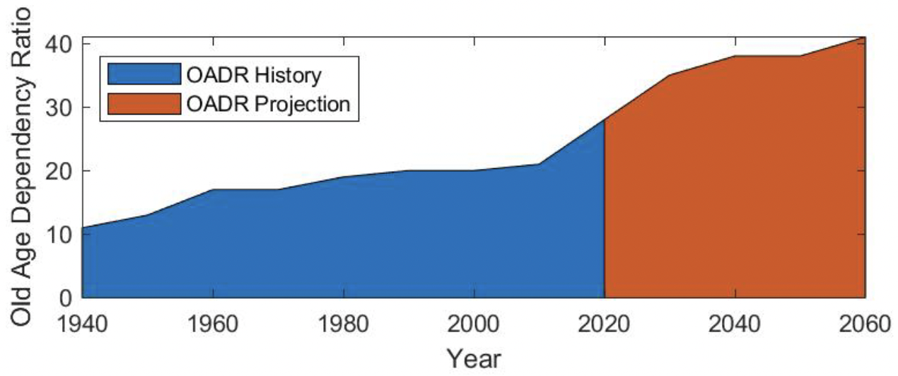
With the exception of the baby boom, the last 100 years has experienced a general decline in the birth rate, eventually leading to a declining population growth rate. At the same time as the population growth rate declined, life expectancy increased significantly. Both of these factors shifted the US demographic composition towards a heightened dependency ratio, which increased pending SSTF outlays, contracted the relative tax base, and left policymakers with difficult choices.
Evaluating Fiscal Alternatives
The purpose of the simulations is to measure the trade-off between the old-age insurance benefit of SSTF outlays versus the distortionary taxation costs of the program’s receipts. To that extent, it is beyond the scope of current simulations to evaluate other aspects of the program, like the progressivity of the benefit formula, or limitations on taxable income or earnings calculation. Instead, the focus is on the pure annuity value, whereby the government pools resources to reduce individuals’ risk of exhausting financial resources late in life.
To generate a comparable basis, the simulation projects the optimal Social Security replacement rate, which represents the share of average wages in working years that are replaced by the benefit in retirement. For example, if average earnings over an individual’s lifetime are $60,000, and annual benefits are $21,000, then the replacement rate is 35 percent. By studying how the optimal replacement ratio changes with certain demographic values, such as longer life spans and declining population growth rate, the results can be translated into policy guidance.
To understand how the optimal replacement rate responds to demographic changes, the simulations are broken down into two sets – those corresponding to life expectancy changes over the last century, and those corresponding to changes in the population growth rate. The ongoing assumption is that population weights corresponding to these demographic combinations are stable. While current demographics are certainly in transition, this assumption allows for simpler calculations that provide an approximation to current trends.
Figure 2 — Optimal Replacement Rate as It Relates to Survival Probabilities by Cohort and the Population Growth Rate
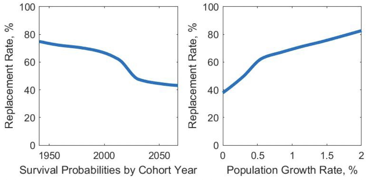
Over the last century, survival probabilities have generally increased for each age and each new cohort in the US. The left graph in Figure 2 shows how the optimal replacement ratio has changed with the evolution of survival probabilities for the cohorts spanning 1940-2065.7 Since an increase in survival probabilities expands the program’s outlays relative to its contributions, the net effect is an increase in outlays. In response, the optimal replacement ratio drops from about 75 percent for the early cohorts down to 43 percent for cohorts that will be born in 2065.8,9 The graph flattens out for cohorts born around 2020 and after because life expectancy is expected to stabilize.
So long as increases in the population growth rate materialize through increases in the share of younger cohorts, possibly through a heightened fertility or younger-aged immigration, then the program’s receipts increase relative to the outlays. This means that the optimal replacement ratio should rise as the population growth rate increases. The right graph in Figure 2 shows exactly this relationship. As the population growth rate increases, the optimal replacement ratio roughly doubles from about 40 percent to 82 percent.
While it may seem hopeful that an increasing population growth rate could support a higher benefit, population projections show a different trajectory. The last several decades have seen a sharp decline in the population growth rate from 1.7 percent in 1960 to 0.6 percent in 2018.10 The problem only seems to compound over the foreseeable future as the fertility rate continues to decline.
Although the model recommends a decline in the benefit provision in each case (as they relate to trending demographics), the direction of the tax change is mixed. In the case of the rising life expectancy, the model suggests an increase of about 2.4 percentage points relative to current Social Security tax rates, while it recommends actually decreasing the tax rate about roughly 1 percentage point relative to current taxes as the growth rate of the population declines from 2 percent to 0 percent.
To understand this result, consider the effects of these demographic changes on the costs and benefits of the program. In each case, the costs of the program rise, prompting a scale-back in the benefit. In only the case of improved life expectancy, however, do the benefits of the program also rise. Since people live longer lives in that scenario, the annuity value of the benefit increases. By contrast, when the population growth rate declines, the costs spread out over a narrower base, but the annuity value of the benefit remains the same. Consequently, this scenario results in both a declining benefit and a declining tax rate.11
Conclusion
Over the last several decades, the US has experienced a considerable increase in life expectancy at the same time as the population growth rate steadily declined. These two demographic transitions contributed to a persistent surge in the retiree dependency ratio, putting a strain on the Social Security system. Under current law and current demographic projections, the SSTF will eventually become insolvent, rendering the current provision unsustainable in the long-run. To bring the program into balance, the simulation model points to sizable reductions in the Social Security replacement ratio. The proposed direction of a tax change, however, was ambiguous, showing sensitivity to the specific driver of demographic changes.
Although the results showed how the Social Security provision should respond to changing demographics, it also implicitly highlighted the opportunity for demographic policies to resolve fiscal imbalances. For example, heightened immigration rates could generate increases in the Social Security tax base that accommodate a more stable benefit. Similarly, any policies that can improve fertility rates might also improve the fiscal outlook of the program.
The projected insolvency of the SSTF is one component of a larger fiscal problem in the US. The Congressional Budget Office anticipates that under current law, government debt is expected to rise to 144 percent of gross domestic product by 2049. If Social Security outlays were limited to the funds generated by the program under current law, then the federal debt projection would fall considerably to 106 percent of gross domestic product.12 As a result, resolving the Social Security ensures the stability of the US government pension program and makes long strides towards resolving the overall federal fiscal outlook.
Appendix
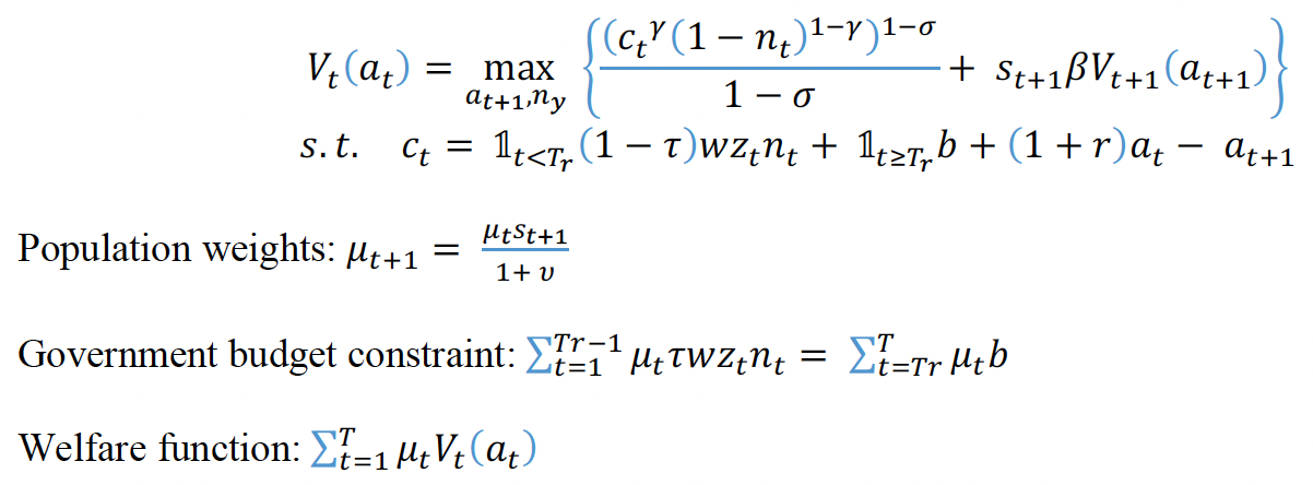
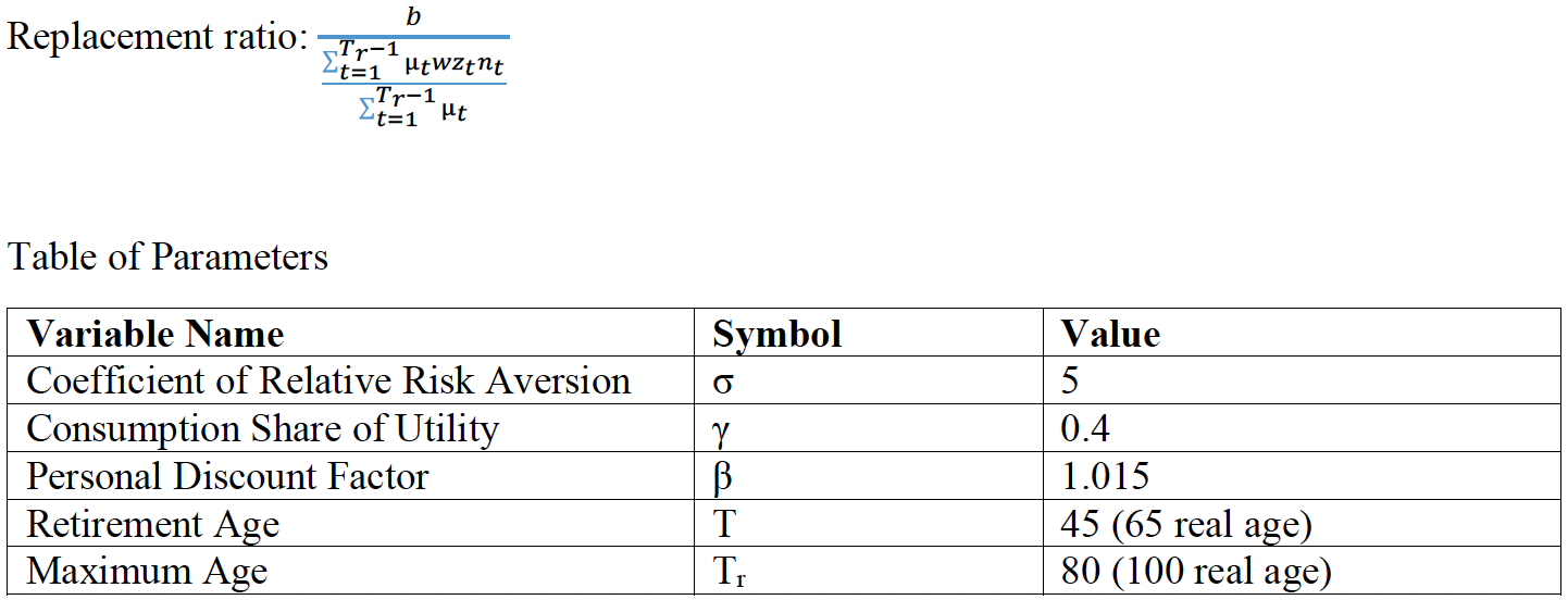
The simulated economy is a standard overlapping-generations model in partial equilibrium, or equivalently, in an open economy. Wages (w) are normalized to unity and the net real interest rate (r) is set to 2 percent. The Bellman equation below characterizes the value function Vt of household at age t with stock of assets at. The household values consumption ct and leisure (1-nt), where nt is labor supply. Households choose over (positive) future assets (at+1) and labor supply (nt) in every period in order to maximize remaining lifetime utility. The government levies a proportional labor income tax (τ) that finances all Social Security expenditures (b) characterized by the government budget constraint below. The parameters υ and st are, respectively, the population growth rate and the probability of a household surviving from age t to age t+1. These two are the only parameters that change across all counterfactual experiments. The remaining parameters are summarized in the table below, with the exception of age-dependent productivity (zt), which changes hyperbolically throughout the household’s working years.
Macroeconomic Simulation Model
Endnotes
1. https://www.ssa.gov/policy/docs/ssb/v70n3/v70n3p111.html
2. Social Security Act of 1935 (Act of August 14, 1935) [H.R. 7260], Titles I-V, X. Accessed July 1, 2019, https://www.ssa.gov/history/35actinx.html
3. Social Security Act of 1939 [H.R. 6635] (PUBLIC-No. 379-76th Congress, Chapter 666-1st Session), Title II Section 202 (a)-(g). Accessed July 12, 2019, https://www.ssa.gov/history/pdf/1939Act.pdf
4. “Historical Background and Development of Social Security: Social Security Benefit Increases 1950-2013.” Social Security Administration, accessed July 1, 2019, https://www.ssa.gov/history/briefhistory3.html
5. 1975 Annual Report of the Board of Trustees of the Federal OASDI Trust Funds, U.S. Government Printing Office, May 6, 1975, accessed July 12, 2019, https://www.ssa.gov/oact/TR/historical/1975TR.pdf
6. “Summary of P.L. 98-21, (H.R. 1900), Social Security Amendments of 1983-Signed on April 20, 1983.” Social Security Administration, accessed July 1, 2019, https://www.ssa.gov/history/1983amend.html
7. Probabilities are estimated for cohorts and ages that have not yet been directly measured. These estimates are provided by the Social Security Administration.
8. Simulations of alternative survival probabilities require an assumption for the population growth rate, which is chosen to be 1 percent.
9. Benchmark replacement ratios are high relative to some estimates of the average in the US. This follows from the optimality of the benchmark replacement rate, which may overstate the real value.
10. https://data.worldbank.org/indicator/SP.POP.GROW?locations=US
11. It should be noted that the optimal tax rate increases as the population growth rate declines from 2 percent to 0.5 percent. Further declines in the population growth rate, however, generate declines in the optimal tax rate.
12. https://www.cbo.gov/system/files/2019-06/55331-LTBO-2.pdf
This material may be quoted or reproduced without prior permission, provided appropriate credit is given to the author and Rice University’s Baker Institute for Public Policy. The views expressed herein are those of the individual author(s), and do not necessarily represent the views of Rice University’s Baker Institute for Public Policy.


